In this article, we talk feature selection for forecasting. We start by explaining why you should
think twice before adding features to your forecasts; then we talk
about some ways to do feature selection for forecasting models. To put things in practical terms, we demo
a feature selection method that has a decent balance between performance and computational
cost in R.
Why you should think twice before including features in your forecasting models?
For many data science models, the more features (often referred to as regressors in forecasting), the better your model accuracy will be. But forecasting is quite finickity, and this is often not the case.
Why is this?
We’ll break this down into a few points.
-
Let’s imagine you want to forecast whether a coin will land heads or tails. That’s going to be a non-starter. This is because the variable you’re trying to forecast (let’s call it the target), is completely random. Some targets just don’t have any signal at all, or don’t have any regressors that provide any signal.
-
Let’s call the observations of the variable you have already seen the actuals. These will often contain a surprising amount of information already. The forecasting algorithm you’re using will be hell bent on picking up on this signal. Which means your feature doesn’t just have to be correlated with the target, it has to provide information that the actuals don’t. This is much rarer. For example, ice cream sales will be correlated with the weather, but it definitely won’t contain any more information than in the actuals.
-
You either need to know your regressor ahead of time (it needs to be forward facing), or you need to forecast that regressor as well. Going back to the ice cream example, this regressor is not forward facing. So if you want to know the weather a week from now, you’ll have to forecast ice cream sales ahead by a week, and then feed that into your forecasting algorithm. This adds a lot of noise to your regressor, which in turn adds noise to your forecast and makes it worse. It is rarely worth doing.
-
Even forward facing regressors frequently add unintended noise to your forecast, just because there is not enough signal, similar to points 1 and 2.
Some ways to perform feature selection for a forecasting algorithm
There are a few ways to check if a regressor provides any useful information to a forecast. Most of these rely on a walkforward backtest. A walkforward backtest is where you start at a historic date (called the train upto date), you forecast using only data up to that date, then you move up to the next date and repeat, until you reach the present.
Then to evaluate your forecast, you can calculate the forecast error compared with actuals. So it is a lot like a train/test set split in classic data science problems. A tutorial of this technique is here. If you have two forecasts you want to decide between, you can run a backtest for each of them. The one with the lowest error would be classed as the best.
With this, here are some ways to perform feature selection, in order of increasing computational and time cost:
1. Look at correlations between the actuals and the regressor.
This just checks the regressor using in-sample fit, and does not cover point 2 in the previous section (does the regressor contain information the forecast doesn’t). This option is not recommended.
2. Use the Akaike Information Criterion (AIC) of the forecast.
This is a statistical approximation that tries to use insample fit to approximate predictive fit. See this chapter for using the AIC for model selection.
The way this would work is you would fit your forecasting model both with and without the regressor, and check the AIC of each. The model with the lowest AIC would be the one you would pick.
This method is good, fast, and commonly used. But it is an approximation that only uses insample fit, so may not give a good estimate of predictive fit.
3. Use linear regression on the actuals with both the current forecast and your regressor as a feature
The key to this method is getting around point 2. We want to check how much additional predictive information our regressor gives after taking into account the information the forecast has learned.
For this method we run a single backtest using the current forecast without regressors. Then we feed both the regressor and the forecast through a linear regression that is trying to learn the actuals.
To assess how good the regressor is, we can examine whether the regressor is significant in the standard way you would assess a linear regression (i.e. check its p-value is sufficiently small). Because we have also included the forecast itself in the regression, this regression should account for what is already learned by the forecasting algorithm.
This method assesses predictive fit directly, but only needs to run one backtest. The method works particularly well when you have many regressors to check. You still just have to fit one backtest (the current forecast with no regressors), then you can use standard techniques for model selection in linear regression, such as recursive feature elimination (make sure you don’t eliminate your forecast though)!
4. Run a forecast backtest with and without the regressor
This method is quite simple, we run a backtest both with a forecast using the regressor, and without. We then compare the error of the two. If the error of the forecast with the regressor is significantly lower, we might use that regressor going forward.
Backtests are bread and butter of model selection in forecasting. So this method works well.
But as the number of regressors goes up, this method gets prohibitively expensive. We have to fit multiple forecasting models on each of the train upto dates.
Demoing method 3
We choose to demo method 3, as it offers a good balance between directly measuring predictive quality of a regressor, with computational cost. Often a backtest of the best forecasting method so far is already at hand from other experiments, which is the most computationally demanding part of this method.
To demo this practically, we’ll use R. Follow along with the interactive Rmarkdown for this tutorial on my github. For all the packages used in
this tutorial, download the FPP3
package
by running in R install.packages('fpp3'). This package is a
companion to the amazing introductory forecasting
book by Rob Hyndman.
The data we’ll use, is the US consumption expenditure data from the
book. This is a time series of quarterly percentage changes of various
measures in the US economy. The one we’re interested in forecasting is
economic production, which is a measure of the health of the US economy.
It can be accessed after loading in fpp3, and is called us_change.
The column we want to forecast is Production. Let’s plot it
library(fpp3)

us_change %>%
    autoplot(Production) +
    labs(y = "Production (% change)")
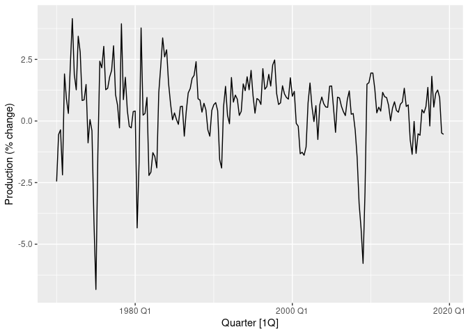
Plot of US % change production over time.
To forecast this data, we’ll fit an ARIMA model to this data, which allows regressors to be added.
To fit the linear regression on the features we need to check, we’ll
need to run a backtest on our forecasting algorithm with no regressors.
Let’s backtest our forecasting model on the last 50 data points, and
forecast one-step ahead. The ARIMA function will automatically perform
parameter tuning for the ARIMA model using AIC.
# Set seed for reproducibility
set.seed(13)
backtest_size <- 50
n <- nrow(us_change)
backtest_results <- us_change[(n - (backtest_size - 1)):n,]
backtest_results$forecast <- rep(NA, backtest_size)
for (backtest_num in backtest_size:1) {
    fit <- us_change[1:(n - backtest_num),] %>%
        select(Production) %>%
        model(
            forecast = ARIMA(Production)
        )
    backtest_fc <- fit %>% forecast(h = 1)
    results_index <- backtest_size - (backtest_num - 1)
    backtest_results$forecast[results_index] <- backtest_fc$.mean
}

# Let’s plot our backtest results against actuals

backtest_results %>%
    pivot_longer(c(Production, forecast), names_to = "Type") %>%
    autoplot(value)
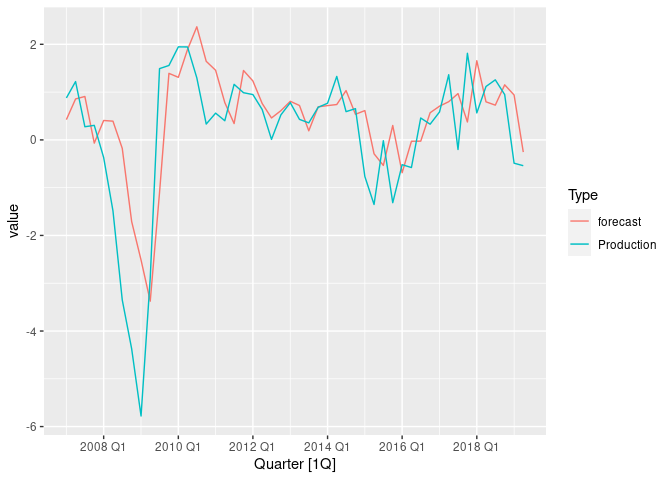
Plot of ARIMA backtest without regressors.
Notice that the forecast does fine during normal periods, but performs poorly during periods of large fluctuation. Can we use regressors to improve this?
We have modelled production data, which is typically measured using GDP.
But measuring GDP takes an enormous effort, and in many countries is
only done every quarter. Other data can be easier to estimate more
regularly, and is more readily available. One measure this might be true
for is consumer spending. This is the Consumption column in our
dataset.
Let’s use a simple linear regression to see if using consumption as a regressor has any promise.
regress_test <- lm(Production ~ forecast + Consumption, data = backtest_results)
summary(regress_test)

##
## Call:
## lm(formula = Production ~ forecast + Consumption, data = backtest_results)
##
## Residuals:
##     Min      1Q  Median      3Q     Max
## -2.4347 -0.7459  0.1566  0.5379  2.4470
##
## Coefficients:
##             Estimate Std. Error t value Pr(>|t|)
## (Intercept)  -0.8588     0.1889  -4.545 3.84e-05 ***
## forecast      0.8750     0.1406   6.224 1.23e-07 ***
## Consumption   1.2630     0.3158   4.000 0.000223 ***
## ---
## Signif. codes:  0 '***' 0.001 '**' 0.01 '*' 0.05 '.' 0.1 ' ' 1
##
## Residual standard error: 0.9268 on 47 degrees of freedom
## Multiple R-squared:  0.6461, Adjusted R-squared:  0.6311
## F-statistic: 42.91 on 2 and 47 DF,  p-value: 2.501e-11
The p-value is very low for the Consumption column, well below the
classic 0.05 level. This indicates including it in the forecast should
improve predictive performance.
What about consumer savings (the Savings column in the dataset)?
regress_test_savings <- lm(Production ~ forecast + Savings, data = backtest_results)
summary(regress_test_savings)

##
## Call:
## lm(formula = Production ~ forecast + Savings, data = backtest_results)
##
## Residuals:
##     Min      1Q  Median      3Q     Max
## -3.1353 -0.5435  0.1223  0.6092  2.7229
##
## Coefficients:
##             Estimate Std. Error t value Pr(>|t|)
## (Intercept) -0.34043    0.16657  -2.044   0.0466 *
## forecast     1.08637    0.14867   7.307  2.8e-09 ***
## Savings     -0.01165    0.01029  -1.132   0.2633
## ---
## Signif. codes:  0 '***' 0.001 '**' 0.01 '*' 0.05 '.' 0.1 ' ' 1
##
## Residual standard error: 1.059 on 47 degrees of freedom
## Multiple R-squared:  0.5383, Adjusted R-squared:  0.5186
## F-statistic: 27.39 on 2 and 47 DF,  p-value: 1.299e-08
The p-value in this case is high, so we should not include savings in our model.
Let’s check our choice by including consumption in the ARIMA model and running a new backtest
backtest_regressor_results <- backtest_results
backtest_regressor_results$forecast_consumption <- rep(NA, backtest_size)
for (backtest_num in backtest_size:1) {
    fit <- us_change[1:(n - backtest_num),] %>%
        select(Quarter, Production, Consumption) %>%
        model(
            forecast = ARIMA(Production ~ Consumption)
        )
    new_regressor <- select(us_change[n - (backtest_num - 1),], Quarter, Consumption)
    backtest_fc <- fit %>% forecast(new_data = new_regressor)
    results_index <- backtest_size - (backtest_num - 1)
    backtest_regressor_results$forecast_consumption[results_index] <- backtest_fc$.mean
}

# Plot both backtests
backtest_regressor_results %>%
    pivot_longer(c(Production, forecast, forecast_consumption), names_to = "Type") %>%
    autoplot(value)
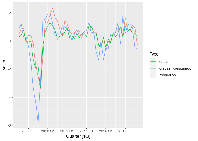
Plot of ARIMA backtest with and without selected regressors.
It’s a little difficult to tell which forecast performed better by eye, so let’s check the MSE error
backtest_regressor_results %>%
    as_tibble() %>%
    summarise(
        MSE_no_regressors = mean((Production - forecast)^2),
        MSE_consumption_regressor = mean((Production - forecast_consumption)^2)
    )

## # A tibble: 1 x 2
##   MSE_no_regressors MSE_consumption_regressor
##               <dbl>                     <dbl>
## 1              1.20                      1.01
The MSE is lower in the backtest including consumption as a regressor, so we probably made the right choice :).
Key Points
- In forecasting, including features are not guaranteed to improve model performance, so think carefully before you do.
- Feature selection in forecasting is a trade off between selection performance and computational cost.
- A way to select features in forecasts that directly measures predictive performance, is to run a backtest of your forecast without regressors, then fit a linear regression model to learn actuals given your forecasts and the regressor. Select the regressor if the p-value is low.